Мы можем использовать метод Кейна для интегрирования уравнений движения для системы n маятников с произвольными массами и длинами ( см. ). Реализация программы вдохновлена jakevdp . Однако, когда я использую этот метод аппроксимации, чтобы найти псевдовременный период T (определенный как среднее всех периодов времени для каждого маятника в системе n маятников, то есть average(period(theta_1),...,period(theta_n))), график T как функция n кажется невероятно отключенным с точки зрения амплитуды.
Цель: визуализировать взаимосвязь между числом маятников n и псевдовременным периодом T=2π/omega bar всей системы, где omega bar является средним значением всех угловых скоростей omega.
Следующая реализация определяет и решает уравнения движения для системы n маятников, с произвольными массами и длинами (в этом случае мы разрешим m[i]=1 для всех i). Это начальная проблема с theta_1(0)=135,...,theta_n(0)=135 и theta_1'(0)=0,...,theta_n'(0)=0.
# %matplotlib inline
import matplotlib.pyplot as plt
import numpy as np
import pandas as pd

from sympy import symbols
from sympy.physics import mechanics

from sympy import Dummy, lambdify
from scipy.integrate import odeint


def integrate_pendulum(n, times,
                   initial_positions=135,
                   initial_velocities=0,
                   lengths=None, masses=1):
"""Integrate a multi-pendulum with `n` sections"""
#-------------------------------------------------
# Step 1: construct the pendulum model

# Generalized coordinates and velocities
# (in this case, angular positions & velocities of each mass)
q = mechanics.dynamicsymbols('q:{0}'.format(n))
u = mechanics.dynamicsymbols('u:{0}'.format(n))

# mass and length
m = symbols('m:{0}'.format(n))
l = symbols('l:{0}'.format(n))

# gravity and time symbols
g, t = symbols('g,t')

#--------------------------------------------------
# Step 2: build the model using Kane's Method

# Create pivot point reference frame
A = mechanics.ReferenceFrame('A')
P = mechanics.Point('P')
P.set_vel(A, 0)

# lists to hold particles, forces, and kinetic ODEs
# for each pendulum in the chain
particles = []
forces = []
kinetic_odes = []

for i in range(n):
    # Create a reference frame following the i^th mass
    Ai = A.orientnew('A' + str(i), 'Axis', [q[i], A.z])
    Ai.set_ang_vel(A, u[i] * A.z)

    # Create a point in this reference frame
    Pi = P.locatenew('P' + str(i), l[i] * Ai.x)
    Pi.v2pt_theory(P, A, Ai)

    # Create a new particle of mass m[i] at this point
    Pai = mechanics.Particle('Pa' + str(i), Pi, m[i])
    particles.append(Pai)

    # Set forces & compute kinematic ODE
    forces.append((Pi, m[i] * g * A.x))
    kinetic_odes.append(q[i].diff(t) - u[i])

    P = Pi

# Generate equations of motion
KM = mechanics.KanesMethod(A, q_ind=q, u_ind=u,
                           kd_eqs=kinetic_odes)
fr, fr_star = KM.kanes_equations(particles, forces)

#-----------------------------------------------------
# Step 3: numerically evaluate equations and integrate

# initial positions and velocities – assumed to be given in degrees
y0 = np.deg2rad(np.concatenate([np.broadcast_to(initial_positions, n),
                                np.broadcast_to(initial_velocities, n)]))

# lengths and masses
if lengths is None:
    lengths = np.ones(n) / n
lengths = np.broadcast_to(lengths, n)
masses = np.broadcast_to(masses, n)

# Fixed parameters: gravitational constant, lengths, and masses
parameters = [g] + list(l) + list(m)
parameter_vals = [9.81] + list(lengths) + list(masses)

# define symbols for unknown parameters
unknowns = [Dummy() for i in q + u]
unknown_dict = dict(zip(q + u, unknowns))
kds = KM.kindiffdict()

# substitute unknown symbols for qdot terms
mm_sym = KM.mass_matrix_full.subs(kds).subs(unknown_dict)
fo_sym = KM.forcing_full.subs(kds).subs(unknown_dict)

# create functions for numerical calculation
mm_func = lambdify(unknowns + parameters, mm_sym)
fo_func = lambdify(unknowns + parameters, fo_sym)

# function which computes the derivatives of parameters
def gradient(y, t, args):
    vals = np.concatenate((y, args))
    sol = np.linalg.solve(mm_func(*vals), fo_func(*vals))
    return np.array(sol).T[0]

# ODE integration
return odeint(gradient, y0, times, args=(parameter_vals,))
Выше приведены обобщенные физические координаты, то есть угловое положение theta и скорость omega каждого сегмента маятника относительно вертикали. Далее извлекаются координаты (x,y) из обобщенных координат.
def get_xy_coords(p, lengths=None):
    """Get (x, y) coordinates from generalized coordinates p"""
    p = np.atleast_2d(p)
    n = p.shape[1] // 2
    if lengths is None:
        lengths = np.ones(n) / n
    zeros = np.zeros(p.shape[0])[:, None]
    x = np.hstack([zeros, lengths * np.sin(p[:, :n])])
    y = np.hstack([zeros, -lengths * np.cos(p[:, :n])])
    return np.cumsum(x, 1), np.cumsum(y, 1)
Затем мы фиксируем число маятников, скажем, n=10 и определяем период псевдо-времени следующим образом:
n = 10
nperiod = []
#Array containing pseudo-period for a system of `n` pendulums
for i in range(1,n + 1):
t = np.linspace(0, 10, 1000)
p = integrate_pendulum(i, times=t)
#x, y has first column of zeros
x, y = get_xy_coords(p)
r,s = np.shape(y)
#Call method to find pseudo-period
nperiod.append(computeperiod())
#Takes `j`, denoting `j`-th pendulum, as input and returns `theta_j` for all times where `1≤j≤n`. This information corresponds to the `j`-th column of the `y` matrix, transformed into polar coordinates.
def theta(j):
theta_j = []
for i in range(0, r):
theta_j.append(math.acos(abs(y[i][j-1]-y[i][j])))
#We should technically divide by the length of the pendulum in `abs(.)`
timenew = [i for i in range(1,r + 1)]
graph_j = pd.Series(data=theta_j, index=timenew)
#Returns array omega_j which is the numerical time derivative of all values contained in the `r x 1` array `theta_j`, i.e. the value of the `j`-th angle theta_j for all times
return pd.Series(data=np.gradient(graph_j.values), index=graph_j.index)
#Returns pseudo-time period using formula `T=2π/omega`
def computeperiod():
series = []
for j in range(1,s):
series.append(2 * math.pi/(theta(j).mean()))
numberline = [i for i in range(1,s)] #Here s=n+1
timeperiod = pd.Series(data=series, index=numberline)
return abs(timeperiod.mean())
print(nperiod)
numbers = [i for i in range(len(nperiod))]
finalperiods = pd.Series(data=nperiod, index=numbers)
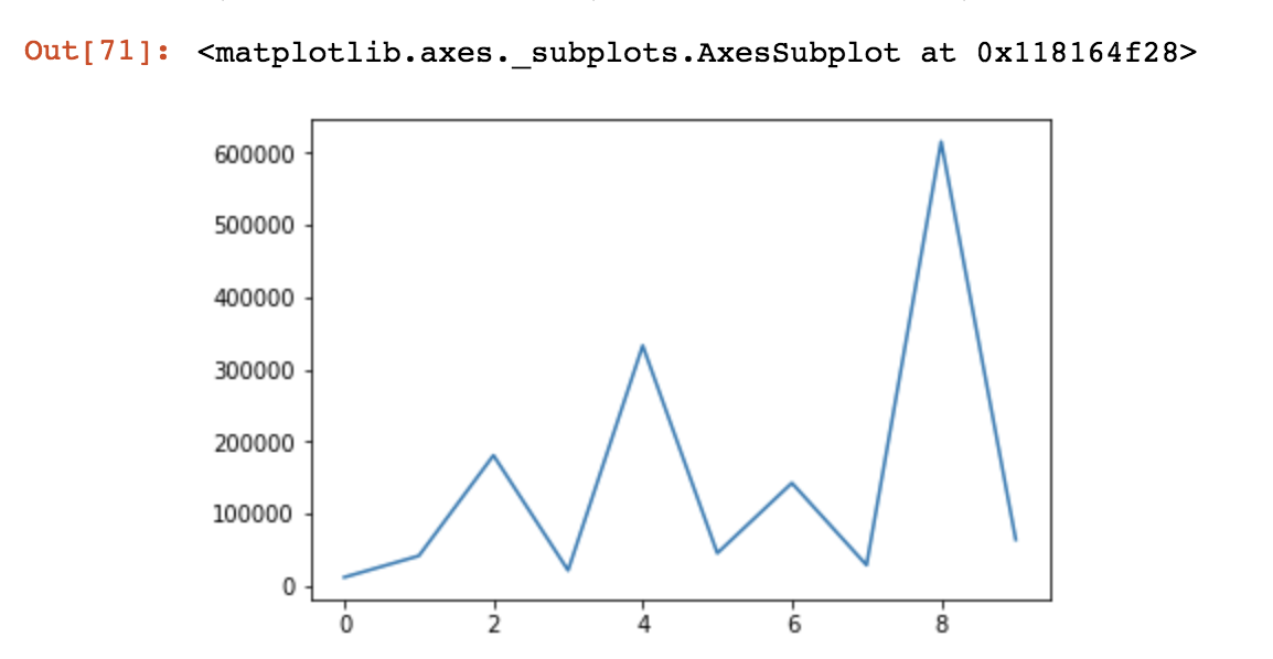
finalperiods.plot()
Когда мы строим его, мы получаем следующий график для n=10:
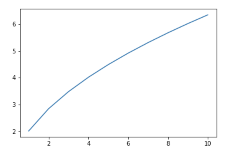
 Однако он должен вести себя асимптотически как
 O(n^(3/2)) в соответствии с T(n) = 2 * π * n^(3/2)(l/g)^(1/2), где g = 9.8 и l = 1, как показано ниже.
Кроме того, его амплитуда должна быть уменьшена примерно в 100,000. Таким образом, кажется, что с этим методом что-то явно не так.