В агентском проекте моделирования я подумывал использовать tidyverse a tibble вместо matrix.Я проверил эффективность обоих с очень простой ПРО (см. Ниже), где я моделирую население, где люди стареют, умирают и рождаются.Типично для ПРО, я использую цикл for и индексацию.
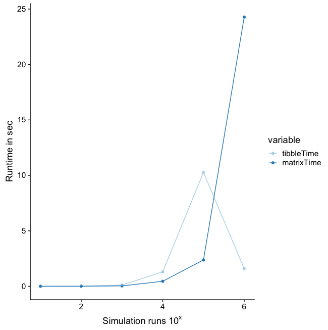
При сравнительном анализе двух структур данных (см. График здесь: https://github.com/marcosmolla/tibble_vs_matrix) матрица намного быстрее, чем тиббл. Однако для прогонов 10e6 этот результат фактически инвертируется. И я понятия не имею,почему.
Было бы здорово понять этот результат, чтобы сообщить, буду ли я использовать тиблы или матрицы в будущем для этого вида использования.
Спасибо всем за любой вклад!
# This code benchmarks the speed of tibbles versus matrices. This should be useful for evaluating the suitability of tibbles in a ABM context where matrix data is frequently altered in matrices (or vectors).

library(tidyverse)
library(reshape2)
library(cowplot)

lapply(c(10^1, 10^2, 10^3, 10^4, 10^5, 10^6), function(runtime){
  # Set up tibble
  indTBL <- tibble(id=1:100,
         type=sample(1:3, size=100, replace=T),
         age=1)

  # Set up matrix (from tibble)
  indMAT <- as.matrix(indTBL)

  # Simulation run with tibble
  t <- Sys.time()
  for(i in 1:runtime){
    # increase age
    indTBL$age <- indTBL[["age"]]+1

    # replace individuals by chance or when max age
    dead <- (1:100)[runif(n=100,min=0,max=1)<=0.01 | indTBL[["age"]]>100]
    indTBL[dead, "age"] <- 1
    indTBL[dead, "type"] <- sample(1:3, size=length(dead), replace=T)
  }
  tibbleTime <- as.numeric(Sys.time()-t)

  # Simulation run with matrix
  t <- Sys.time()
  for(i in 1:runtime){
    # increase age
    indMAT[,"age"] <- indMAT[,"age"]+1

    # replace individuals by chance or when max age
    dead <- (1:100)[runif(n=100,min=0,max=1)<=0.01 | indMAT[,"age"]>100]
    indMAT[dead, "age"] <- 1
    indMAT[dead, "type"] <- sample(1:3, size=length(dead), replace=T)
  }
  matrixTime <- as.numeric(Sys.time()-t)

  # Return both run times
  return(data.frame(tibbleTime=tibbleTime, matrixTime=matrixTime))
}) %>% bind_rows() -> res

# Prepare data for ggplot
res$power <- 1:nrow(res)
res_m <- melt(data=res, id.vars="power")

# Line plot for results
ggplot(data=res_m, aes(x=power, y=value, color=variable)) + geom_point() + geom_line() + scale_color_brewer(palette="Paired") + ylab("Runtime in sec") + xlab(bquote("Simulation runs"~10^x))